To run the models in cerebmodels the user must be in the root of ``~/cerebmodels/``
Since this notebook is in ~/cerebmodels/docs/notebooks/ the user must move up two directories
[1]:
cd ..
/home/main-dev/cerebmodels/docs
[2]:
cd ..
/home/main-dev/cerebmodels
Model Execution - Case1: no stimulation, raw-mode (i.e. without evoking capability)
1. Set-up
Import ExecutiveControl of cerebmodels
[3]:
from executive import ExecutiveControl as ec
2. Search for models and pick a desired model
2.1. See available model scales
[4]:
ec.list_modelscales()
[4]:
['subcell', 'synapses', 'cells', 'microcircuits', 'layers']
2.2. See available models for a particular scale
Below shows the available models at the level of cellular modelling scale.
[5]:
ec.list_models( modelscale = "cells" )
[5]:
['PC2010Genet',
 'GoC2007Solinas',
 'GrC1994Gabbiani',
 'PC2009Akemann',
 'PC2013Marasco',
 'PC2006Akemann',
 'GoC2010Botta',
 'PC2001Miyasho',
 'PC2003Khaliq',
 'GoC2011Souza',
 'GrC2016Dover',
 'PC2018Zang',
 'PC1997aHausser',
 'PC2015Masoli',
 'PC2011Brown',
 'PC2015aForrest',
 'GrC2011Souza',
 'PC2015bForrest',
 'GrC2001DAngelo',
 'PC1997bHausser',
 'DCN2011Luthman',
 'GrC2009Diwakar']
2.3. Pick a desired model
Although it is not essential to instantiate ExecutiveControl to launch the model, it is recommended if one were to visualize the response.
[6]:
exc = ec()
[7]:
%%capture
desired_model = exc.choose_model( modelscale = "cells", modelname = "PC2003Khaliq")
3. Launching (executing) the desired model
3.1. Setting the parameters
For our cases of launching the model without stimulation and without CerbUnit’s capability, one is just required to define the run-time parameters.
[8]:
runtimeparam = { "dt": 0.025, "celsius": 37, "tstop": 500, "v_init": -65 }
3.2. Executing the model
[9]:
desired_model = exc.launch_model(parameters = runtimeparam, onmodel = desired_model )
--- 0.15529299999999946 seconds ---
3.3. Saving the response
In CerebUnit the model response are saved in an HDF5 file based on NWB:2.0 scheme. Execution of save_response() returns the filename and its path. Below, this return full path and filename is assigned to the attribute ``fullfilename`` of the model.
[10]:
%%capture
desired_model.fullfilename = exc.save_response()
4. Visualizing the response
4.1. List model regions of the chosen model
Before one calls the visualization function the user must define the the region of interest (roi) from which the response will be visualized.
[11]:
exc.list_modelregions( chosenmodel = desired_model )
[11]:
['soma v']
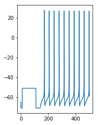
4.2. Visualize all events
The method visualize_all plots all the events in respective sub-plot. In our particular case with not stimulation the simulation has only one event therefore only one sub-plot is seen below.
[12]:
exc.visualize_all(chosenmodel = desired_model, roi="soma v")
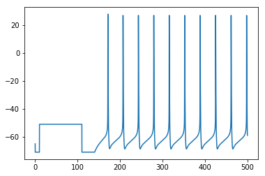
4.3. Visualize all events in one plot
[13]:
exc.visualize_aio(chosenmodel = desired_model, roi="soma v")
[ ]: